Introduction

A core principle in machine learning is the bias-variance trade-off, which describes the balance between model complexity and how well a model generalizes to unseen data. Traditionally, model error on test data is expected to follow a U-shaped curve. If the model is too simple it fails to capture actual trends or patterns in the data (large bias). As we increase the model size, test performance begins to improve as the model learns underlying patterns in the data. However, if the model becomes too complex it begins to fit random noise and spurious patterns specific to the training sample, poorly generalizing to unseen data (large variance). As the number of model parameters \(P\) approaches the size of the training dataset \(N\), the model reaches the interpolation threshold and gains enough degrees of freedom to fit the training data perfectly. While the model can perfectly fit the training data at this point, it generalizes poorly to new, unseen data. Beyond this point we expect model error to continue to grow as model complexity increases and the model becomes increasingly sensitive to noise and spurious patterns in the training set. The optimal model size lies somewhere between underfitting and overfitting, being complex enough to capture true structure in the data, but not so flexible that it learns random noise. This trade-off is a core concept that is taught in all introductory machine learning courses.

However, the success of overparameterized neural networks over recent years seems to defy this traditional piece of wisdom and calls into question the universality of the bias-variance trade-off. Recent studies have observed that as model size increases, test error initially rises, peaking at around the interpolation threshold, but then enters a new regime that exhibits a second descent in test error. This “double descent” was first detailed by Belkin et al. (2019). They found double descent also occurs in linear regression, trees, and boosting models. Follow-up work by OpenAI also showed this double descent extends to epoch-wise and data-wise double descent. In epoch-wise double descent training longer can initially hurt and later improve test performance; in data-wise double descent, adding more data can sometimes worsen generalization before it improves again!

In many cases, pushing beyond the interpolation threshold doesn’t just recover performance, but often leads to models that outperform those from the initial descent phase. This surprising behavior has led to a shift in the prevailing wisdom, particularly in the context of deep learning, where the current wisdom seems to be that “bigger is better”. This phenomenon represents one of the most intriguing open areas in modern machine learning. Why do largely overparameterized models generalize so well, despite having the capacity to memorize training data? A deeper understanding of this behavior has significant implications, not just for a theoretical understanding, but for how we design, train, and deploy models in real-world applications.

In this post, I aim to take a closer look at double descent and review some recent findings in demystifying what is going on. I illustrate the phenomenon with a simple synthetic linear regression example, and show how an effective measure of complexity introduced by Curth et al. (2023) recovers the classic U-shaped bias-variance trade-off curve. I conclude with some thoughts on what we’ve learned, what are some remaining open questions, and where future work might lead in exploring this interesting area of research.

The code to recreate the analyses in this post is available on GitHub.

Exploring double descent with linear regression

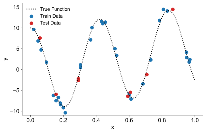
To get a better picture of the double descent phenomenon, I give a simple example inspired by Schaeffer et al. (2023), using polynomial regression. In this setup, we generate data according to the relation:
\[ y = 2x + 3\textrm{cos}(15x) + \epsilon \] where the noise term \(\epsilon\) is drawn from a normal distribution \(\epsilon \sim \textrm{Normal}(0,1)\). We sample 40 data points from the relation, with inputs \(x_i\) drawn uniformly from the unit interval \(x_i \sim [0,1]\). The data is then randomly split into test and training sets, with 80% (32 data points) used for training and 20% (8 points) reserved for testing. The resulting dataset is shown in the figure below.

To model the data, we use polynomial regression. Specifically, we map each input \(x_i\) to a \(P\)-dimensional feature space, with the feature maps \(\boldsymbol{\phi} : \mathbb{R} \rightarrow \mathbb{R}^P\), where each \(\phi_p\) corresponds to the \(p^\textrm{th}\) Legendre polynomial. We then fit a linear model \( \hat{y_i} = \sum_{p=1}^P \beta_p \phi_p (x_i) \), with \(\boldsymbol{\beta} = (\beta_1, …, \beta_P)^T\) representing the \(P\) regression coefficients.

We define \(\Phi\) to be the design matrix, given as \[ \Phi = \begin{pmatrix} \phi_1 (x_1) & \phi_2 (x_1) & \dots & \phi_P (x_1) \\ \phi_1 (x_2) & \phi_2 (x_2) & \dots & \phi_P (x_2) \\ \vdots & \vdots & \ddots & \vdots \\ \phi_1 (x_N) & \phi_2 (x_N) & \dots & \phi_P (x_N) \end{pmatrix}\] and denote by \(\boldsymbol{y} = (y_1, …, y_N)^T\) the vector of observed outputs for the \(N\) training points.

To infer values for \(\boldsymbol{\beta}\), we then solve the classical least-squares minimization problem: \[ \boldsymbol{\beta} := \textrm{arg} \min_{\boldsymbol{\beta}} || \Phi \boldsymbol{\beta} - \boldsymbol{y} ||^2 \] which minimizes the squared error between the model predictions and the observed outputs.

However, when the model is overparameterized (\(P > N\)), the optimization problem becomes ill-posed, since we have fewer data constraints than parameters. This leads to infinitely many solutions that can perfectly fit the training data. To resolve this, we instead solve a different (constrained) optimization problem, and solve for the smallest parameters \(\boldsymbol{\beta}\) that guarantee \(\boldsymbol{\Phi}\boldsymbol{\beta} = \boldsymbol{y}\):

\[ \boldsymbol{\beta_{\textrm{over}}} := \textrm{arg} \min_{\boldsymbol{\beta}} || \boldsymbol{\beta} ||_2^2 \quad \textrm{s.t.} \quad \boldsymbol{\Phi} \boldsymbol{\beta} = \boldsymbol{y} \]

This approach yields the minimum-norm interpolating solution, which is the same optimization problems used in recent work investigating double descent: Belkin et al. (2019), Schaeffer et al. (2023), Curth et al. (2023).

To see the double descent phenomenon, we fit models with increasing model complexity, varying the number of parameters \(P\) from 1 to 200, and plot the resulting train and test root mean square errors (RMSE).

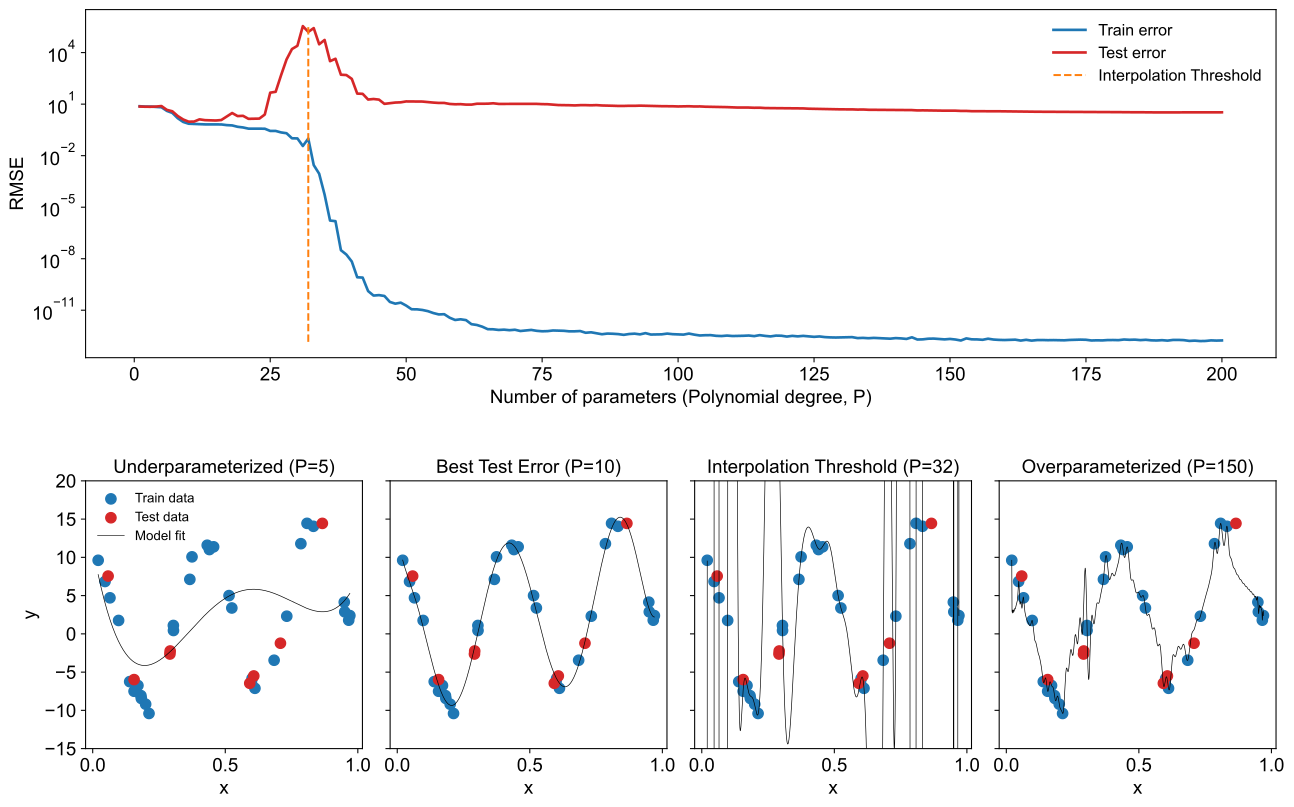
The figure above displays training and test RMSE in the top panel, and example model fits in the bottom panels, illustrating underfitting, best fit, interpolation threshold, and overparameterized regimes.

As we increase model complexity, we see training error steadily decreases and converges to zero error beyond the interpolation threshold. Meanwhile, test error initially decreases and then rises sharply near the interpolation threshold (exhibiting the classic U-shaped bias-variance trade-off). However, beyond this point, we see test error decreases again, resulting in a second descent. In this toy example, the best-performing model still happens to lie in the lower-complexity region (\(P<N\)), but that isn’t always the case. In many real-world settings, overparameterized models often outperform simpler ones, with studies showing that the best generalization error can occur well beyond the interpolation threshold. Nonetheless, even in this simple example we see a clear instance of double descent.

So what’s going on here? Looking at representative fits from each scenario helps to form a better picture. When \(P \ll N\), training and test errors are both high due to underfitting. The model lacks enough flexibility to capture patterns in the data, as seen for \(P=5\) in the figure above. At \(P=10\), the model captures the underlying structure well, balancing flexibility and avoiding noise. Approaching the interpolation threshold, the model fits training data perfectly but generalizes poorly, and becomes erratic between training data points. At this point, there is only one model that lowers the train error optimally, with no wiggle room. It is therefore very sensitive to noise in the data. Unless the data is noise-free and the model class happens to match the true function exactly (which is highly unlikely), this will generally lead to poor test performance. However, as we continue to increase the model size, the fit begins to smooth out. It is still able to perfectly fit the training data, but behaves better in between. As a result, the test error begins to improve again. But why does this extra “smoothing” emerge?

A U-turn on double descent?

Rethinking parameter counting: Why not all complexity is equal

You might have noticed something strange in how we defined the optimization problem above. For the overparameterized case (\(P>N\)), we switched to a different formulation! This change is necessary to make the problem well-posed and yield a unique solution. But isn’t it curious that this is also the point where double descent seems to kick in? Coincidence? Probably not.

In fact, Curth et al. (2023) argue it’s not a coincidence at all. They argue that when we change the way we solve the model in the overparameterized (\(P>N\)) setting, we’re actually performing an implicit form of unsupervised dimensionality reduction. The main idea is that, even as the number of raw features grows, the solution is still constrained to the \(N\)-dimensional row space of the feature matrix \(\boldsymbol{\Phi}\). So the model only sees a space shaped by the training inputs \(\boldsymbol{x}_{\textrm{train}}\). This is similar to projecting the data onto a lower-dimensional space, as in principle component analysis (PCA), and performing the regression there. It’s unsupervised, because the projection depends only on the inputs. This reveals a key insight. There are actually two distinct ways to increase parameter count. When \(P \leq N\), adding features increases the model capacity directly. When \(P>N\), adding more features doesn’t increase the number of parameters that can be fit using supervised learning, there are still only \(N\) parameters that are effectively determined by the data. Instead, the additional features enhance the expressiveness of the input representation through an unsupervised process. Stay tuned for a follow-up post that explores this in further detail.

Curth et al. (2023) also show that there are distinct ways in which parameters can be increased in decision tree and boosting models. For example, if we increase the number of leaves per tree (i.e., make each model more flexible), we get the usual U-shaped curve. But if we fix the leaf size and instead increase the number of trees in the ensemble, test error keeps dropping with no second rise. Therefore, the shape of the test error curve depends on which parameters are increased, and not all parameters are created equal. Accordingly, they show that the second descent is not inherently tied to the interpolation threshold, and they can even get multiple descents by alternating how each parameter type is increased.

Measuring effective model complexity and getting back to U

Its clear that simply counting raw parameters (e.g \(P\)) can be misleading and not actually capture model complexity. To get a more meaningful measure, Curth et al. (2023) derived an effective measure of model complexity motivated by previous definitions developed for smooothers. Smoothers are a class of supervised learning methods where predictions are formed by averaging (or “smoothing”) over training outputs: \[\hat{f}(x_0) = \mathbf{s}(x_0) \cdot \boldsymbol{y_\textrm{train}} = \sum_{i \in I_{\textrm{train}}} s_i (x_0) y_i\] Here, \(\mathbf{s}(x_0)\) are smoothing weights that determine how much each training output \(y_i\) influences the prediction at the point \(x_0\). Building on previous definitions for effective number of parameters, the authors define a variance-based effective parameter measure: \[ p_e = \frac{N}{|I_0|} \sum_{j \in I_0} ||\mathbf{s}(x^0_j) ||^2 \] where \(I_0\) is a set of points (e.g. test or training data). This quantity captures how sensitive predictions are to perturbations in the training outputs. See Appendix for a derivation of smoothing weights and \(p_e\) for linear regression.

Let’s see how this measure applies to our polynomial regression example. For each fitted model, we compute the effective number of parameters, \(p_e\), using the formula above on test data, and plot the test RMSE against this measure.

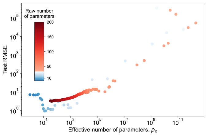
In the figure above, we replot the test RMSE, this time against the effective number of parameters. Unlike the raw parameter count, with this new measure, we see that we do indeed see the classical U-shaped curve, where with few parameters the model underfits, then reaches a “sweet spot”, and then continues to increase in error as the effective number of parameters increases.

We also look at how the effective number of parameters compares to the actual raw number of parameters, corresponding to the polynomial degree, \(P\). Interestingly, we see that as the raw number of parameters increases, the effective number of parameters increase too, up until we reach the interpolation threshold, which is where the problem formulation changes. After this, increasing the raw number of parameters actually decreases the number of effective parameters! Therefore, we see the inductive bias of minimum norm actually leads to effectively lower model complexity as we increase \(P\), allowing the model to fit the data and generalize well to unseen data.

Concluding thoughts

Re-examining model complexity and double descent

Curth et al. (2023) offer a more nuanced explanation of double descent. They show that there may be multiple distinct ways to increase model parameters, with not all parameters being equal. Their key insight is that how we increase model parameters matters, and can lead to qualitatively different generalization behavior. This distinction between ways to increase model complexity plays a key role in explaining the second descent. Moreover, they show effective model complexity is not always aligned with nominal complexity (e.g., the raw parameter count). When looking at the effective complexity of the model, we see that we recover the classical U-shaped curve, and there is no second descent.

What does this mean in practice? First, we should be aware that model complexity is not a one-dimensional concept. In the cases explored by Curth et al. (2023), there are two axes of complexity. Increasing along the first axis, (number of leaves per tree, number of regression basis functions, or number of boosting iterations), increases the model’s ability to fit the training data and reduces bias. Increasing along the second axis helps reduce variance at test time by smoothing predictions, e.g. by averaging over more weak learners or aggregating across more basis functions or projections. Model error tends to be more sensitive to hyperparameter tuning along the first axis, while increasing along the second axis mainly improves performance. Interestingly, increasing parameters along the second axis may also make the model less sensitive to the first axis. So in improving model performance, bigger might be better, but now we have a better understanding of why and when that is the case.

It is also important to understand the inductive biases present in the model, whether explicit or implicit. We see in linear regression, the minimum-norm bias seems to be a good one in improving model generalizability. While we didn’t discuss deep double descent in detail here, one main idea is that optimization algorithms such as stochastic gradient descent, implicitly regularize parameters to be low norm, and this might in part explain why large neural networks often generalize well despite their size.

Open questions and future directions

Double descent has drawn the most attention in the context of deep learning. However there are still many open questions on double descent in this setting.

One area of interest is the role of implicit regularization. In deep learning, stochastic gradient descent has been shown to lead to low-norm or low-complexity solutions, but the exact mechanisms and details are still unclear. What kinds of functions are we exactly biasing towards and how consistent is this across architectures, tasks, and datasets? Perhaps if we understood this better, we can design explicit regularization strategies or model architectures that better leverage these principles to improve models.

It is also not clear exactly what the conditions are that lead to double descent. How universal is this phenomenon and how does it depend on model architecture, data distribution, level of noise, or training dynamics?

Beyond this, one of the most compelling hypotheses from deep learning research is that larger models enable the learning of more generalizing features. As discussed in this Anthropic post, smaller or underparameterized models may rely on memorizing training examples, encoding them as features in superposition. As model capacity or dataset size increases, these networks may learn more structured feature representations that can improve generalization. This shift from memorizing data to discovering deeper underlying structure may help explain the second descent in test error. This process also seems to resemble how adding more parameters allows linear regression models to develop a richer basis and capture deeper structure in the data.

One of the most important open questions, in my opinion, is: What biases guide overparameterized models to discover meaningful features (i.e. those that are tied to semantic meaning, causality, or structure), rather than superficial correlations? Understanding this could be key to designing models that don’t just fit data effectively, but also reason robustly and generalize reliably. It might even help us better understand how humans learn and reason by revealing why certain features or patterns appear interpretable, meaningful, or semantically rich to us.

Thanks for reading! The code to recreate the analyses in this post is available on GitHub and can be run directly in Google Colab. I’m always looking to improve these posts. If you have feedback or questions, feel free to email me, open a GitHub issue, or connect with me on LinkedIn!

References

1. Curth, Alicia, Alan Jeffares, and Mihaela van der Schaar. “A u-turn on double descent: Rethinking parameter counting in statistical learning.” Advances in Neural Information Processing Systems. (2023)
2. Belkin, Mikhail, et al. “Reconciling modern machine-learning practice and the classical bias–variance trade-off.” PNAS. (2019)
3. Schaeffer, Rylan, et al. “Double descent demystified: Identifying, interpreting & ablating the sources of a deep learning puzzle.” arXiv preprint. (2023)
4. Nakkiran, Preetum, et al. “Deep double descent: Where bigger models and more data hurt. Journal of Statistical Mechanics: Theory and Experiment. (2021)
5. Henighan, Tom et al. “Superposition, Memorization, and Double Descent” Transformer Circuits Thread. (2023)

Appendix

Derivation of smoothing weights and number of effective parameters for linear regression

To derive the smoothing weights for linear regression, we start by equating the prediction of a smoother with that of the linear regression model. A smoother is expressed as: \[\hat{f}(x_0) = \mathbf{s}(x_0)^T \boldsymbol{y_\textrm{train}}\] for any admissible input \(x_0\), where \(\mathbf{s}(x_0)\) is the smoothing weight vector applied to the training targets \(\boldsymbol{y_\textrm{train}}\).

In linear regression, the model prediction at test point \(x_0\) is given by: \[ \hat{f}(x_0) = \boldsymbol{\phi}(x_0)^T \boldsymbol{\beta} \] where \(\boldsymbol{\phi}(x_0) = (\phi_1 (x_0), \dots \phi_P (x_0))\) is the feature vector at \(x_0\), and \(\boldsymbol{\beta}\) is the vector of regression coefficients. Equating the two expressions gives: \[ \mathbf{s}(x_0)^T \boldsymbol{y_\textrm{train}} = \boldsymbol{\phi}(x_0)^T \boldsymbol{\beta}\] The least squares solution for \(\boldsymbol{\beta}\) depends on the shape of the design matrix \(\boldsymbol{\Phi}_\textrm{train}\) (with rows \(\boldsymbol{\phi}(x_i)^T\), for each training example \(x_i\)). Depending on the shape, we have:

• Underparameterized case (\(P < N\)): \[ \boldsymbol{\beta} = (\Phi^T_{\textrm{train}}\Phi_{\textrm{train}})^{-1} \Phi^T_{\textrm{train}}\mathbf{y}_{\textrm{train}}\]
• Overparameterized case (\(P \geq N\)), using the minimum-norm solution: \[ \boldsymbol{\beta} = \Phi^T_{\textrm{train}} (\Phi_{\textrm{train}}\Phi^T_{\textrm{train}})^{-1} \mathbf{y}_{\textrm{train}}\]

Substituting back into the prediction expression above, we can identify the smoothing weights as:

• For \(P < n\): \[\mathbf{s}(x_0)^T = \boldsymbol{\phi}(x_0)^T (\Phi^T_{\textrm{train}}\Phi_{\textrm{train}})^{-1} \Phi^T_{\textrm{train}}\]
• For \(P \geq n\): \[ \mathbf{s}(x_0)^T = \boldsymbol{\phi}(x_0)^T \Phi^T_{\textrm{train}} (\Phi_{\textrm{train}}\Phi^T_{\textrm{train}})^{-1} \]

The derivation assumes the identity holds for any choice of \(\mathbf{y}_{\textrm{train}}\), allowing us to equate the coefficient matrices directly and extract the smoothing weights.

Given smoothing weights \(\mathbf{s}(\boldsymbol{x}^0)\) for some set of inputs \(x_j^0\) for \({j \in I_0}\), the “Generalized effective number of parameters” \(p_e(\boldsymbol{x}^0)\) as defined in Curth et al. (2023), is given as \[ p_e = \frac{N}{|I_0|} \sum_{j \in I_0} || \mathbf{s} (x_j^0) ||^2 \]

If we denote by \(\mathbf{S_0}\) the matrix with rows \(\mathbf{s} (x_j^0)\), for each \(x_j^0\), we can express this as \[ p_e = \frac{N}{|I_0|} \textrm{tr} (\mathbf{S_0} \mathbf{S_0^\textit{T}} )\]